Layer On this page A layer is a function that transforms input
Basics Linear# What: linear transformation
Why: Universal Approximation Theorem
Notations:
Dropout# $$
Y=\mathrm{Dropout}(X, p)
$$
Idea: randomly make some elements become 0 with specified probability
Notations:
Residual Block (ResNet)# $$
Y\leftarrow Y+X
$$
Idea: add input to output
reduce vanishing gradient problem allow parametrization for the identity function
add complexity in the simplest way Normalization# Batch Normalization# $$
Y=\gamma\frac{X-E_m[X]}{\sqrt{\mathrm{Var}_m[X]+\epsilon}}+\beta
$$
Idea: normalize each feature independently across all samples
Notations:
Pros:
Allow us to use higher learning rates Allow us to care less about param initialization Cons:
Dependent on batch size
Layer Normalization# $$
Y=\gamma\frac{X-E_n[X]}{\sqrt{\mathrm{Var}_n[X]+\epsilon}}+\beta
$$
Idea: normalize each sample independently across all features
Notations:
Pros:
Same as BN Applicable on small batches
CNN Convolution# $$
Y_{ij}=\sum_{c=0}^{C_{in}-1}W_{jc}\ast X_{ic}+\textbf{b}_j
$$
Idea: convolution
Notations:
Pooling# Max Pooling# $$
Y_{ijhw}=\max_{u\in[0,H_{filt}-1]}\max_{v\in[0,W_{filt}-1]}X_{ij,H_{filt}*h+u,W_{filt}*w+u}
$$
Idea: pool images by selecting the max element in each filter window (the equation is stupid, just visualize it)
Notations:
Average Pooling# $$
Y_{ijhw}=\frac{1}{H_{filt}W_{filt}}\sum_{u=0}^{H_{filt}-1}\sum_{v=0}^{W_{filt}-1}X_{ij,H_{filt}*h+u,W_{filt}*w+u}
$$
Idea: pool images by selecting the max element in each filter window (the equation is stupid, just visualize it)
Notations:
NiN block (Network in Network)# Idea: 1
significantly improve computational efficiency while keeping the matrix size and at the same time add local nonlinearities across channel activations
RNN RNN# $$
h_t=\tanh(x_tW_{xh}^T+h_{t-1}W_{hh}^T)
$$
Idea: recurrence - maintain a hidden state that captures information about previous inputs in the sequence
Notations:
Cons:
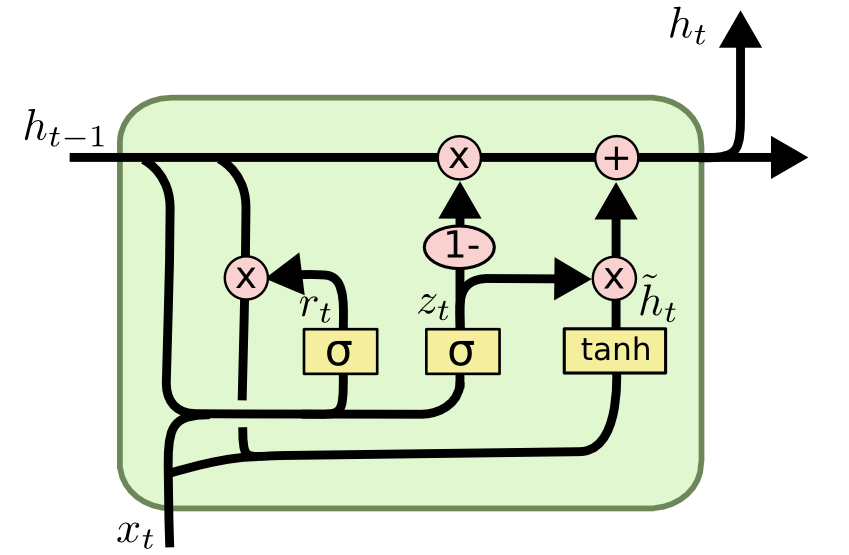
Short-term memory: hard to carry info from earlier steps to later ones if long seq Vanishing gradient: gradients in earlier parts become extremely small if long seq GRU# Idea: Gated Recurrent Unit - use 2 gates to address long-term info propagation issue in RNN:
Reset gate : determine how much of
Update gate : determine how much of
Candidate : calculate candidate
Final : calculate weighted average between candidate
Notations:
LSTM# Idea: Long Short-Term Memory - use 3 gates:
Input gate : determine what new info from
Forget gate : determine what info from prev cell
Candidate cell : create a new candidate cell from
Update cell : use
Output gate : determine what info from curr cell
Final : simply apply
Notations:
What : Transformer exploits self-attention mechanisms for sequential data.
Why :
long-range dependencies : directly model relationships between any two positions in the sequence regardless of their distance, whereas RNNs struggle with tokens that are far apart.parallel processing : process all tokens in parallel, whereas RNNs process them in sequence.flexibility : can be easily modified and transferred to various structures and tasks.Where : NLP, CV, Speech, Time Series, Generative tasks, …
When :
sequential data independence: a sequence can be processed in parallel to a certain extent. importance of contextual relationships importance of high-dimensional representations sufficient data & sufficient computational resources How :
All layers used in transformer: Each sublayer follows this structure:
Input : input/output token embeddings
Encoder : input
Decoder : output
Output : Decoder embeddings
Training :
Parameters :Encoder:
Decoder:
Hyperparameters :#layers hidden size #heads learning rate (& warm-up steps) Inference :
Process input tokens in parallel via encoder. Generate output tokens sequentially via decoder. Pros :
high computation efficiency (training & inference) high performance wide applicability Cons :
require sufficient computation resources require sufficient large-scale data
Positional Encoding# What : Positional Encoding encodes sequence order info of tokens into embeddings.
Why : So that the model can still make use of the sequence order info since no recurrence/convolution is available for it.
Where : After tokenization & Before feeding into model.
When : The hypothesis that relative positions allow the model to learn to attend easier holds.
How : sinusoid with wavelengths from a geometric progression from
For any fixed offset
Pros :
allow model to extrapolate to sequence lengths longer than the training sequences Cons : ???
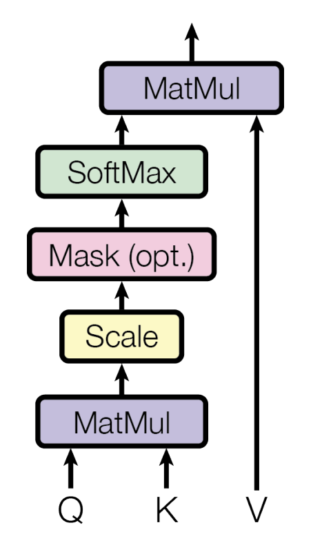
Scaled Dot-Product Attention# What : An effective & efficient variation of self-attention.
Why :
The end goal is Attention - “Which parts of the sentence should we focus on?” We want to capture the most relevant info in the sentence. And we also want to keep track of all info in the sentence as well, just with different weights. We want to create contextualized representations of the sentence. Therefore, attention mechanism - we want to assign different attention scores to each token. When :
linearity : Relationship between tokens can be captured via linear transformation.Position independence : Relationship between tokens are independent of positions (fixed by Positional Encoding).How :
$$
\text{Attention}(Q,K,V)=\text{softmax}(\frac{QK^T}{\sqrt{d_k}})V
$$
Preliminaries:Query (Q) : a question about a token - “How important is this token in the context of the whole sentence?”Key (K) : a piece of unique identifier about a token - “Here’s something unique about this token.”Value (V) : the actual meaning of a token - “Here’s the content about this token.” Procedure:Compare the similarity between the Q of one word and the K of every other word.The more similar, the more attention we should give to that word for the queried word. Scale down by
Dot products grow large in magnitude, pushing the softmax function into regions where it has extremely small gradients. They grow large because, if
Convert the attention scores into a probability distribution .Softmax sums up to 1 and emphasizes important attention weights (and reduces the impact of negligible ones). Calculate the weighted combination of all words, for each queried word, as the final attention score. Pros :
significantly higher computational efficiency (time & space) than additive attention Cons :
outperformed by additive attention if without scaling for large values of
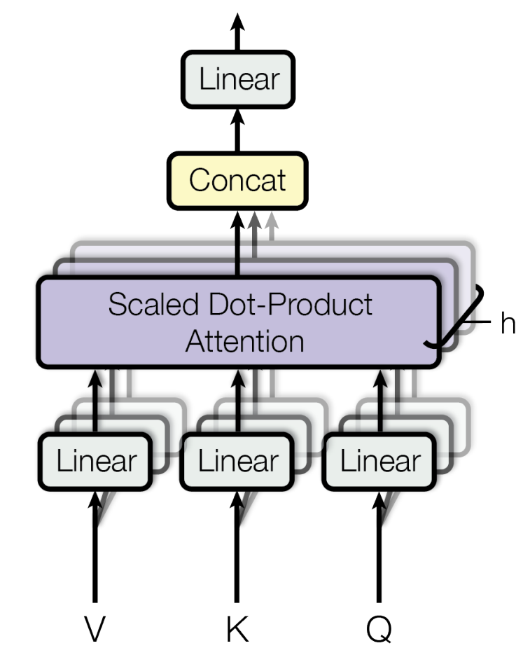
Multi-Head Attention# What : A combination of multiple scaled dot-product attention heads in parallel.
Masked MHA: mask the succeeding tokens off because they can’t be seen during decoding. Why : To allow the model to jointly attend to info from different representation subspaces at different positions.
When : The assumption of independence of attention heads holds.
How :
Pros :
better performance than single head Cons : ???
Postion-wise Feed-Forward Networks# What : 2 linear transformations with ReLU in between.
Why : Just like 2 convolutions with kernel size 1.
How :
$$
\text{FFN}(x)=\max(0,xW_1+b_1)W_2+b_2
$$
 into output
 .
.


 : input tensor of arbitrary shape
 : output tensor of the input shape
 : dropout probability


 : (hyperparam) batch size
 : (hyperparam) #features
 : (hyperparam) tiny value to avoid zero division
 : (learnable param) init as 1
 : (learnable param) init as 0
 ineffective for small batches


 : #channels of input, #channels of output
 , height and width of output (image)
 : padding size
 : stride size
 : sample index
 : out channel index

 : #channels
 (stride size is filter size in pooling)
 1 convs (+ global average pooling)
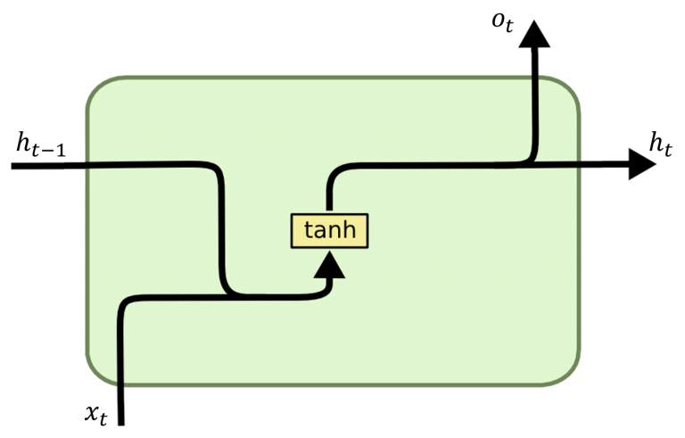


 .
. .
. .
. with the retain ratio.


 : element-wise product
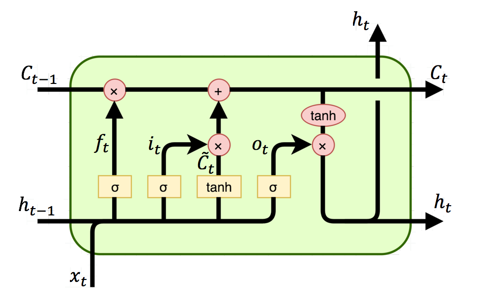

 .
. should be forgotten.
 .
. to combine prev and new candidate cells.
 .
. .
.


 )
)
 input for Encoder/Decoder
 for Decoder
 Decoder embeddings
 token probabilities


 : absolute position of the token
 : dimension
 .
.
 to avoid the similarity scores being too large.
 .
.

 : learnable linear projection params.
 : learnable linear combination weights.
 in the original paper.
