Optimization

Loss

Loss is a measure of difference between predicted output .

• Unreduced loss:
• Reduced loss: $\mathcal{L}(\mathbf{y},\mathbf{\hat{y}})=\begin{cases} \text{sum}(\mathcal{L})=\sum_{i=1}^{m}l_i\\ \text{mean}(\mathcal{L})=\frac{1}{m}\sum_{i=1}^{m}l_i \end{cases}$ (can impose sample weights as well)

Regression#

L1 (Absolute Error)#

Pros:

• Robust to outliers

Cons:

• Non-differentiable
• Less related to the underlying assumption of Gaussian distribution on the errors (for most problems)

L2 (Squared Error)#

$$ \mathcal{l}_i=(y_i-\hat{y}_i)^2 $$

Pros:

• Penalize large errors more heavily
• Differentiable
• Closely related to the underlying assumption of Gaussian distribution on the errors (for most problems)

Cons:

• Sensitive to outliers

Huber#

$$ l_i(\delta)=\begin{cases} \frac{1}{2}(y_i-\hat{y_i})^2 & \text{if }|y_i-\hat{y_i}|\leq\delta\\ \delta|y_i-\hat{y_i}|-\frac{1}{2}\delta^2 & \text{if }|y_i-\hat{y_i}|>\delta \end{cases} $$

Pros:

• A mixture of L1 and L2 losses

Cons:

• Less used than either L1 or L2

Classification#

0-1 (Heaviside)#

$$ l_i=\begin{cases} 0 & \text{if }y_i\hat{y_i}>0\\ 1 & \text{if }y_i\hat{y_i}<0 \end{cases}, y_i\in\{-1,1\} $$

Usage: Naive Bayes

Cons:

• Penalize all incorrect predictions equally
• Non-convex
• Non-differentiable

Hinge#

$$ l_i=\max{(0,1-y_i\hat{y}_i)}, y_i\in\{-1,1\} $$

Usage: SVM

Pros:

• Allow misclassification (penalize more heavily for confident incorrect predictions than for uncertain predictions)
• No penalty on confident correct predictions
• Convex

Cons:

• Non-differentiable at 0

Logistic#

$$ l_i=\frac{1}{\log{2}}\log{(1+e^{-y_i\hat{y_i}})}, y_i\in\{-1,1\} $$

Usage: LogReg

Pros:

• Convex
• Differentiable

Cons:

• Penalize confidently correct predictions
• Penalize confidently incorrect predictions less compared to other losses

Exponential#

$$ l_i=e^{-y_i\hat{y}_i}, y_i\in\{-1,1\} $$

Usage: AdaBoost

Pros:

• Convex
• Differentiable
• Much heavier penalty on much stronger misclassification (effective for weight assignments to examples for AdaBoost)

Cons:

• Penalize confidently correct predictions

Squared#

$$ l_i=(1-y_i\hat{y}_i)^2, y_i\in\{-1,1\} $$

Usage: rare

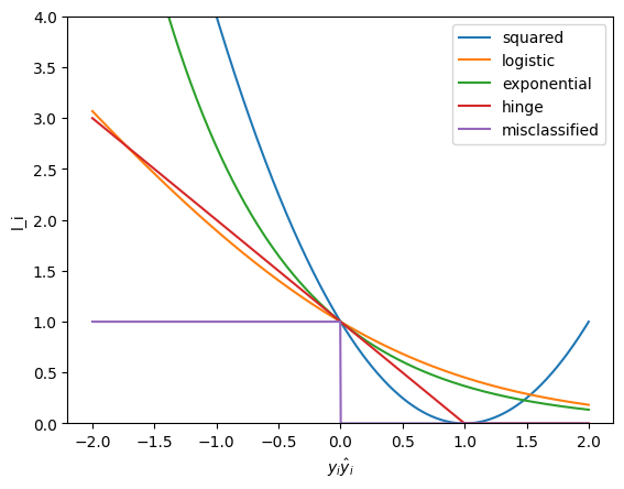
Visualization of all the above losses:

Cross Entropy#

Usage: most (= Log loss for binary, with a much more prevalent label definition)

Pros:

• Extremely easy to compute (all terms become 0 except one)

Cons:

• Sensitive to imbalanced datasets

Kullback-Leibler Divergence (Relative Entropy)#

$$ l_i=y_i\log\frac{y_i}{\hat{y}_i} $$

Usage: anywhere necessary to calculate difference between true and predicted probability distributions (i.e., information loss)

Regularization

• Regularization reduces overfitting by adding our prior belief onto loss minimization (i.e., MAP estimate). Such prior belief is associated with our expectation of test error.
• Regularization makes a model inconsistent, biased, and scale variant.
• Regularization requires extra hyperparameter tuning.
• Regularization has a weaker effect on the model (params) as the sample size increases, because more info become available from the data.

Explicit (Penalty)#

L1#

Pros:

• Sparse Feature selection (reduce weights of trash features to 0)
• Robust to outliers
• Equal weight shrinkage ( )
• Effective with multicollinearity
• Able to handle cases

Cons:

• No closed-form solution (high computational cost with LinReg)
• Need to select perfect

L2#

Pros:

• More/Less shrinkage on larger/smaller weights ( )
• Effective with multicollinearity
• Closed-form solution. Low computational cost with LinReg

Cons:

• No sparsity No feature selection
• Not robust to outliers
• Not able to handle cases
• Need to select perfect

Elastic Net#

$$ \lambda(r_{\text{L1}}||\mathbf{w}||_1+(1-r_{\text{L1}})||\mathbf{w}||_2^2) $$

• : L1 ratio

Pros:

• A mixture of L1 and L2 penalties

Cons:

• Less used than either L1 or L2

L0#

Optimization: Search

• Streamwise Regression:

  1. Init model. Init .
  2. For in range(1,n+1):
     1. Add feature to model.
     2. If :
        1. Keep .
        2. 
     3. Else:
        1. 
  • Pros:
    • Low computational cost:
  • Cons:
    • No guarantee to find optimal solution
    • Order of features matters
      
      

• Stepwise Regression:

  1. Init model. Init .
  2. While True (n loops):
     1. Try to add each of all remaining features to model.
     2. Pick the feature with :
     3. If :
        1. Add feature to model.
        2. 
     4. Else:
        1. Break
  • Pros:
    • More likely to find optimal solution than streamwise
  • Cons:
    • High computational cost:
    • Overfitting
    • Multicollinearity
      
      

• Stagewise Regression:

  1. Init model. Init .
  2. While True (n loops):
     1. Try to add each of all remaining features to model.
     2. Pick the feature with :
     3. If :
        1. Add feature to model. Add to cache.
        2. 
     4. Else:
        1. Break
  • Pros:
    • Faster than stepwise regression (no need to create new long models each time)
    • No multicollinearity
    • Used for boosting
  • Cons:
    • High computational cost:

Common Pros:

• Explicit feature selection Sparsity

Common Cons:

• Severe limitations in optimization methods
• Extreme computational cost

Implicit#

tbd

Parameter Optimization

The word “Learning” in ML is literally just parameter estimation (i.e., objective optimization). Pure statistics.

Gradient Descent#

$$ \boldsymbol{\theta}\leftarrow\boldsymbol{\theta}-\eta\nabla\mathcal{L}(\boldsymbol{\theta}) $$

Types:

• Stochastic GD: update params for each single sample
• Mini-Batch GD: update params for each mini-batch of samples
• Batch GD: update params after observing all samples

Pros:

• Extremely widely used

Cons:

• Cannot find global minimum if
  • bad step size: too big then unstable; too small then taking too long
  • non-convex objective: stuck at local minima or saddle point

Adagrad#

Idea: tune the learning rate so that the model learns slowly from frequent features but pay special attention to rare but informative features. $$ \eta_{tj}=\frac{\eta}{\sqrt{\sum_{\tau=1}^t(\frac{\partial\mathcal{L}_k}{\partial{\theta_j}})^2}+\epsilon} $$

Expectation-Maximization#

Idea: learn model (do MLE/MAP on params) with latent variables (NOT explicit for GMM).

Method:

1. Init params
2. E-step: estimate .
   • Estimate the expected value of the latent variables given the current estimates of the model params and the data.
3. M-step: estimate " (MAP).
   • Estimate the model params through MLE or MAP on the expected value of the complete data likelihood.
4. Repeat Step 2-3 until convergence.

Pros:

• Offer estimates for both latent variables and model params

Cons:

• NOT guaranteed to find optimum

Hyperparameter Tuning

tbd

Evaluation

In regression, MAE/MSE/RMSE is used for both training and evaluation.

In classification, there are various metrics mostly centered at the idea of confusion matrix.

Confusion Matrix#

Confusion Matrix is a matrix which visualizes actual classes against predicted classes.

An example of confusion matrix for binary classification:

• Notations:
  • T&F = whether prediction matches actual
  • P&N = predicted class
  • FP = type 1 error
  • FN = type 2 error
• Metrics:
  • Error Rate:
  • Accuracy:
  • Specificity: TN rate among negative actual values:
  • 1-Specificity (FPR): FP rate among negative actual values:
  • Precision: TP rate among positive predicted values:
  • Recall: TP rate among positive actual values:
  • F-score: harmonic mean of Precision and Recall:
  • F1-score:
• ROC (Receiver Operating Curve): plot of TPR vs FPR
• AUC (Area Under Curve): area under ROC curve

Distance & Similarity

Norm & Distance#

Norm is NOT a distance measure but a size measure. It offers insights for many prevalent distance measures.

Properties:

Types:

Cosine Similarity#

tbd

Kernel#

Def: measure of similarity between 2 vectors.

Properties:

• is positive semi-definite.
  • PSD: .
  • : non-negative real eigenvalues.
  • : real eigenvectors.
• 
• 
• 
• is polynomial func with positive coeffs.
• 
• 
•